More Resources Must Mean Better Outcomes – Right? Or How Variation Can Catch You Out! Part I

Introduction 

This is a two-part blog around variation and the way it can catch people out when attempting cost-cutting exercises or providing additional resources and looking for evidence of benefit. 

In Part I, we’ll look at cost-cutting, as this seems to have been a popular approach, particularly in the Public Sector, to providing “better-value” for Customers and the Public. It is much easier to tell an organisation, or a team, to reduce their budget by 15%, and keep the same level of service, and if service levels drop, then popular argument dictates, “the cuts were too deep” It is much more difficult to provide additional resources and look for hard evidence of an increase in service levels (What size of increase? Any specific parts of the service?). This second approach will be discussed in Part II. 

And some of the points made in Part I will be good background to understanding and getting to grips with Part II. 

Our observations during our travels can be characterised as, “Why, when we have reduced operational costs by only 15% (substitute your own %s), have we seen such a dramatic deterioration in service levels?”  

The answer in many cases is simple to say – “Variation” – but is a much more difficult point to visualise. 

We have developed a simple (compared to the real-world) but sophisticated (in that it can model some complex flows of work) simulation of a generic 4-Stage Business Process to help get understanding across. It’s been developed for educational purposes, and is not a commercially available product. We’ll use some of its output here to hopefully illustrate the point being made. 

We’ll just try to capture the essence of just some of the words and phrases that have been used to describe the world we live and operate in: 

• VUCA (Volatile, Uncertain, Complex and Ambiguous), and a blog can be found here on this subject – https://blogs.cranfield.ac.uk/leadership-management/cbp/military-tactics-and-command-control-fact-or-myth 
• Complex, as described in the CYNEFIN Framework, and a blog can be found here on this subject – https://blogs.cranfield.ac.uk/leadership-management/cbp/computer-says-so-innovation-and-cynefin-first-of-four-on-this-subject-2 
• Indeterministic, meaning the only way to look at the world is through the lens provided by probabilities and statistics, rather than using arithmetic methods (e.g. comparing results from one point in time vs another) 
• Non-linear, meaning that if I change some input parameter (e.g. budget, resources, time-constraint, etc.) in a Business System or Process by X%, then the output from the System might change unpredictably, and certainly not proportionally.  

You’ve probably heard other descriptions which boil down to the same thing. The critical feature is that “Cause & Effect”, “If – Then – Else”, “I do this and expect that” and the like do not work (or work only over very short periods of time) in this environment. And the biggest contributor to this is the hidden Variation – and it’s hidden because many organisations with all the BI tools in the world do not know how to visualise it! 

Now we blogged about the most appropriate well-proven method for visualising Variation over time – using extended-SPC (and not manufacturing-style SPC), see for example https://blogs.cranfield.ac.uk/leadership-management/cbp/why-performance-reporting-is-not-performance-management-part-3 

But, in order to really understand Variation, sometimes it requires that we see it represented in a different way. So let’s turn to the simulation. 

Background to Simulator 

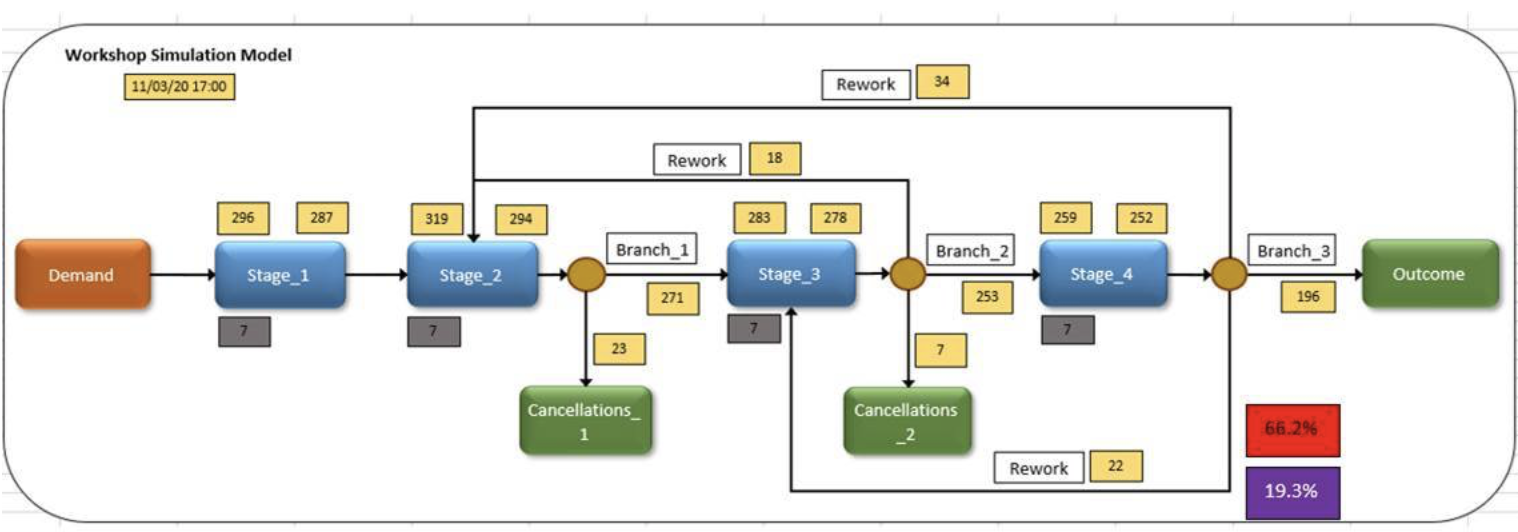
The model represents a generic 4-Stage Business Process (see diagram below). It could be any one or more of Incident Handling in Emergency Services, IT Help Desk, patients passing through a hospital system, new order processing, etc. It is designed to demonstrate many facets of such a System in real life, so for brevity, only a partial description will be provided here. 

In brief demand enters at the left travelling right through the stages or branches into outcomes or cancelations. There are a number of boxes with figures in them representing values that are subject to Variation. We’ll look at a sample simulation run captured in the diagram below. 

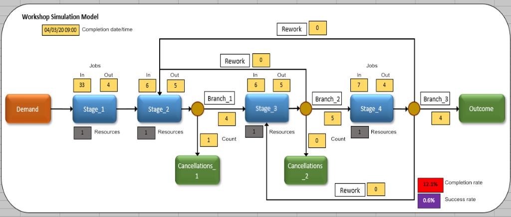
It also makes visible “hidden” Work In Progress (WIP, and, to avoid clutter, is not shown above), that builds up due to Variation, which drives extended Throughout Times.  

The simulation can be set up with a number of “Initial Conditions” – one of which is a Stage by Stage Completion Time Target. We used 10 minutes in the example above. Each Stage Success Rate is the % Jobs completed within Target, and, by multiplying these together for each of the 4 stages, this generates an Overall Success Rate. The simulator also tracks, amongst other parameters, Resource Utilisation (not shown). 

To keep this as simple as possible, we’re going to look at the Overall Completion Rate and the Overall Success Rate for 4 simulation runs, and restricting one element of Variation around Stage Job Completion Time to show how just this one factor can influence performance: 

• Runs 1 and 2 are with, effectively, no Variation in how long it takes to complete a Job at each Stage. Run 1 is with 9 people (Servers) at each Stage, and run 2 is with 7 people at each Stage 
• Runs 3 and 4 are with a small amount of Variation in Stage Job Completion Time, and Run 3 is with 9 people at each Stage, and Run 4 is with 7 people at each Stage. 
•  

Simulation Run 1: No Variation in Job Completion Time: 9 Resources at each Stage 

An Overall Success Rate of 100% might be considered reasonable (or possibly over the top). An Overall Completion Rate of 71.2% might not be, but that question is for another day. With a finance hat on, one might be tempted to look at the Stage by Stage Utilisation rates (not shown) which hover mainly below 60%, and want to drive this number up. After all, one might be able to live with a 20% – 40% reduction from 100% to, say, 60% – 80% Overall Success Rate. Thinking “linearly”, one might therefore reduce the number of Resources by around 20%, to 7 people at each Stage. The results are shown below. 

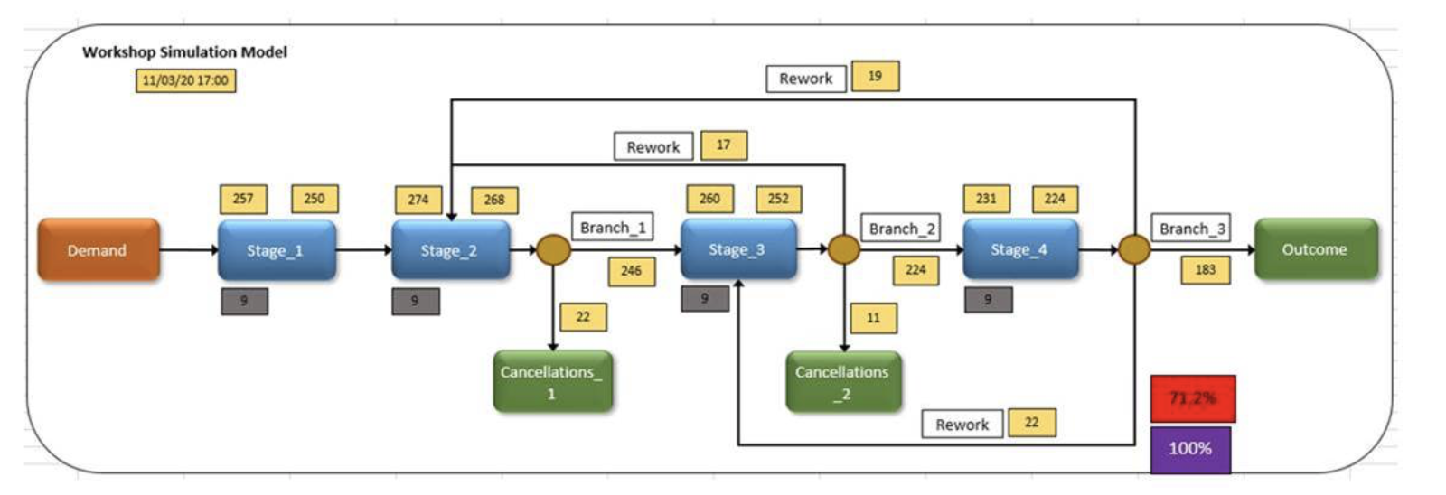
Simulation Run 2: No Variation in Stage Job Completion Time: 7 Resources at each Stage 

Stage Utilisation rates (not shown) have gotten closer to 80% – which might be more satisfactory from a finance point of view. And an Overall Success Rate of 60.6% might be considered OK if we were looking for a range between 60% and 80%. But let’s see what happens when we introduce a small amount of Variation to Job Completion Times. 

Page Break 

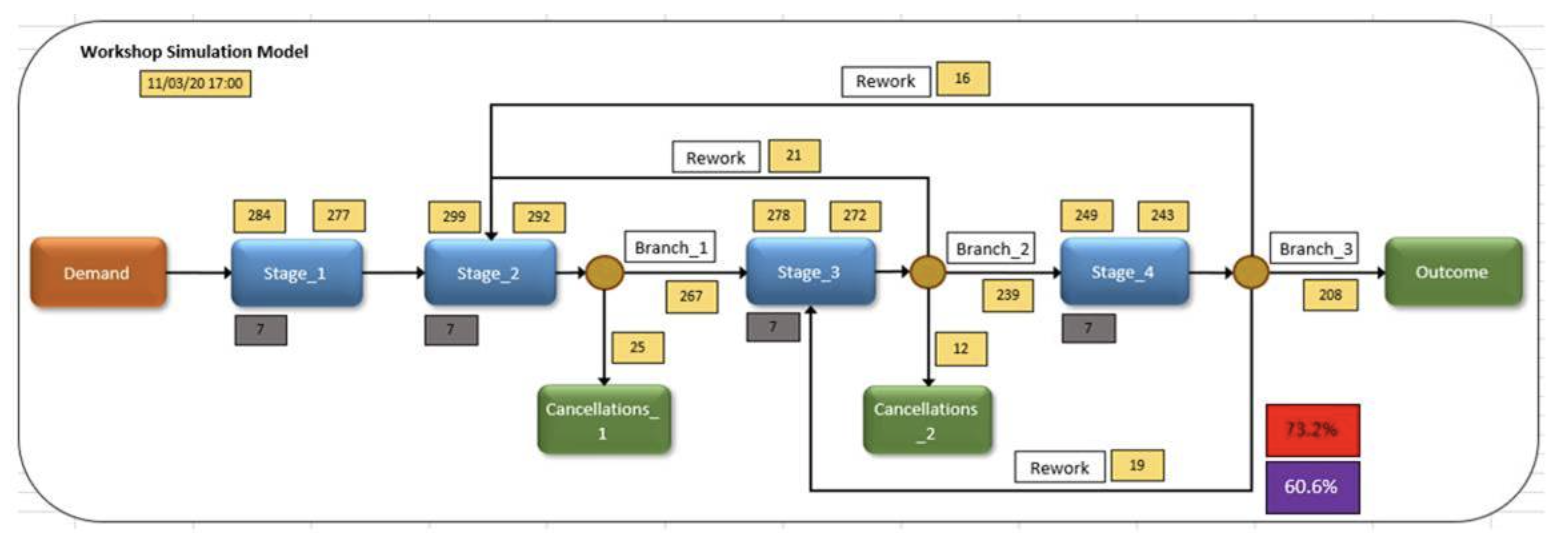
Simulation Run 3: Small Variation in Stage Job Completion Time: 9 Resources at each Stage 

Overall Success Rate is 99.6% vs Simulation Run 1 Overall Success Rate of 100%, and Overall Completion Rate is still up around 70% and above. And, as with Run 1, Utilisation Rates are still below 60%. So what does a cut in Resources of around 20% deliver this time around? 

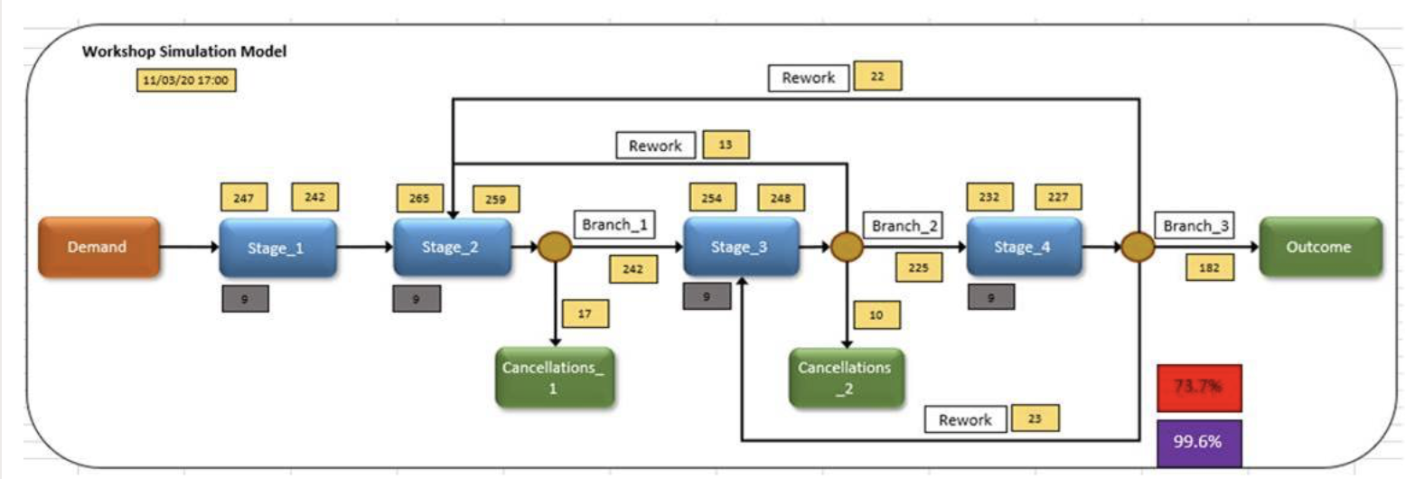
Simulation Run 4: Small Variation in Stage Job Completion Time: 7 Resources at each Stage 

Overall Success Rate has dropped dramatically to 19.3% vs Simulation Run 2 Overall Success Rate of 60.6%. It is this “non-linear” or difficult to predict behaviour when trying to balance Resources with Demand that is the result of hidden Variation, and which nearly always catches people out – laymen and experts alike! 

Now Dominic Cummings knows this – the question is, how many Government Ministers are aware of this? 

Next time we’ll take a look at the converse situation of what to expect when we are adding Resources.